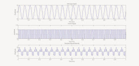
Natural Sampling
In this type of
sampling, the resultant signal follows the natural shape of the input during the
sampling interval.
The sampling
function can be regarded as a form of multiplication. An output occurs when the
input is multiplied by 1, but nothing emerges when it is multiplied by
zero.
 |
| Illustration Of Natural Sampling ( The first Signal is Message Signal, Second one is Carrier & multiplication of which results in Natural Sampled output) |
MATLAB Code for Natural Sampling Illustration
%code starts here
clc;
clear all;
close all;
t = 0:0.001:1; %taking a total of 1000 samples
fc = input('Enter the Frequency of Carrier Signal(square wave) = ');
fm = input('Enter the Frequency of Message Signal(sine wave) = ');
a = input('Enter the Amplitude of Message Signal = ');
vc = square(2*pi*fc*t); % Creating the square wave (Carrier) with unity amplitude
vm = a.*sin(2*pi*fm*t); % Creating the message wave
n = length(vc); % getting the lenght of carrier wave
for i = 1:n
%this loop for projecting the carrier amplitude of -1 & +1 to 0 & +1
if (vc(i)<=0)
vc(i) = 0;
else
vc(i) = 1;
end
end
y = vc.*vm; % Multiplying the carrier & message signal
subplot(3,1,1);
plot(t,vm); % plotting the message signal
xlabel('Time Axis');
ylabel('Amplitude');
title('Message Signal');
subplot(3,1,2);
plot(t,vc); % plotting the carrier signal
xlabel('Time Axis');
ylabel('Amplitude');
title('Carrier Signal');
axis([0 1 0 1.5]);% to set scaling of x & y axis for better visualization
subplot(3,1,3);
plot(t,y);
% plotting the naturally sampled signal thus generated
xlabel('Time Axis');
ylabel('Amplitude');
title('Sampled Signal (Natural)');
axis([0 1 -a-3 a+3]);
% to set scaling of x & y axis for better visualisation
xlabel('Time Axis');
ylabel('Amplitude');
title('Sampled Signal (Natural)');
axis([0 1 -a-3 a+3]);
% to set scaling of x & y axis for better visualisation
Sample Input:
Enter the Frequency of Carrier Signal(square wave) = 100
Enter the Frequency of Message Signal(sine wave) = 20
Enter the Amplitude of Message Signal = 5
Enter the Frequency of Message Signal(sine wave) = 20
Enter the Amplitude of Message Signal = 5
Output(Graph):
 |
| Natural Sampling (MATLAB Implementation) |