MATLAB Implementation of NATURAL SAMPLING, With MATLAB Code

Natural Sampling
In this type of sampling, the resultant signal follows the natural shape of the input during the sampling interval.
The sampling function can be regarded as a form of multiplication. An output occurs when the input is multiplied by 1, but nothing emerges when it is multiplied by zero.

Illustration Of Natural Sampling
Illustration Of Natural Sampling ( The first Signal is Message Signal, Second one is Carrier & multiplication of which results in Natural Sampled output)

MATLAB Code for Natural Sampling Illustration

%code starts here
clc;
clear all;
close all;
t = 0:0.001:1;
%taking a total of 1000 samples
fc = input('Enter the Frequency of Carrier Signal(square wave) = ');
fm = input('Enter the Frequency of Message Signal(sine wave) = ');
a = input('Enter the Amplitude of Message Signal = ');
vc = square(2*pi*fc*t);
% Creating the square wave (Carrier) with unity amplitude
vm = a.*sin(2*pi*fm*t);  % Creating the message wave
n = length(vc); % getting the lenght of carrier wave
for i = 1:n
   
%this loop for projecting the carrier amplitude of -1 & +1 to 0 & +1
    if (vc(i)<=0)
        vc(i) = 0;
    else
        vc(i) = 1;
    end
end
y = vc.*vm;
% Multiplying the carrier & message signal
subplot(3,1,1);
plot(t,vm);
% plotting the message signal
xlabel('Time Axis');
ylabel('Amplitude');
title('Message Signal');
subplot(3,1,2);
plot(t,vc);
% plotting the carrier signal
xlabel('Time Axis');
ylabel('Amplitude');
title('Carrier Signal');
axis([0 1 0 1.5]);
% to set scaling of x & y axis for better visualization
subplot(3,1,3);
plot(t,y);
 
% plotting the naturally sampled signal thus generated
xlabel('Time Axis');
ylabel('Amplitude');
title('Sampled Signal (Natural)');
axis([0 1 -a-3 a+3]);

% to set scaling of x & y axis for better visualisation 

Sample Input:
Enter the Frequency of Carrier Signal(square wave) = 100
Enter the Frequency of Message Signal(sine wave) = 20
Enter the Amplitude of Message Signal = 5

Output(Graph): 

MATLAB Implementation of NATURAL SAMPLING, With MATLAB Code
Natural Sampling (MATLAB Implementation)

0 comments:

Linear Convolution of two Discrete Sequences usng function Using MATLAB Code: With MATLAB code

In mathematics & signal processing, convolution is a mathematical method applied on two functions f and g, producing a third function that is typically viewed as a modified version of one of the original functions.

The digital convolution with sample interval t = 1 is summarized as:
  1. Flip (reverse) one of the digital functions.

  2. Shift it along the time axis by one sample, j.

  3. Multiply the corresponding values of the two digital functions.

  4.  Summationof products from step 3 to get one point of the digital convolution at j.

  5. Repeat steps 1-4 to obtain the digital convolution at all times, j where the digital functions overlap.
For example, let sk = 2, -2, 1 and hk = 1, 3, 1/2, -1. Convolution of these two discrete signals equals 2, 4, -4, 0, 2 1/2, -1


More References about Convulation:


MATLAB Code to Perform Convolution  of two Discrete Sequences using MATLAB conv() Function:

%Code Starts Here
clc;
clear all;
close all;
x1 = input('Enter First sequence x1(n)[] : ');
t1 = input('Enter Origin location Of Sequence x1 : ');
x2 = input('Enter Second sequence x2(n)[] : ');
t2 = input('Enter Origin location Of Sequence x2 : ');
l1 = length(x1); %length of sequence x1
l2 = length(x2); %length of sequence x2
ln = l1+l2-1;
%length of convoluted sequence
y = conv(x1,x2); % performing convolution using conv() function
a = t1+l1-1;
t = t1:a;
subplot(3,1,1);
stem(t,x1);
xlabel('Time');
ylabel('Amplitude');
title('x1');
a = t2+l2-1;
t = t2:a;
subplot(3,1,2);
stem(t,x2);
xlabel('Time');
ylabel('Amplitude');
title('x2');
tn = t1+t2;
a = tn+ln-1;
t = tn:a;
subplot(3,1,3);
disp('Convoluted Sequence ');
disp(y);
% For printing the convulated output in MATLAB command window
stem(t,y);
%  For plotting the convulated output in MATLAB graph window
xlabel('Time');
ylabel('Amplitude');
title('Convoluted Sequence');

Sample Input (As it will be seen in the Command Window) :
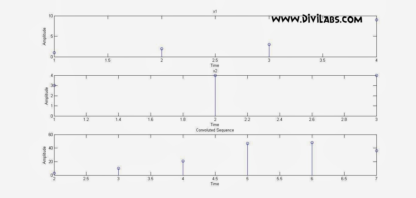
Enter First sequence x1(n)[] : [1 2 3 9]
Enter Origin location Of Sequence x1 : 1
Enter Second sequence x2(n)[] : [3 4 4]
Enter Origin location Of Sequence x2 : 1
Convoluted Sequence
     3    10    21    47    48    36

Graph Thus Obtained: (Containing the 2 input sequences along with the resulted convoluted sequences)

0 comments:

MATLAB Code to Simulate / Generate the Amplitide Modulation Signal (AM Signal) [ Amplitude Modulation using MATLAB]

Amplitude modulation (AM) is a method of superimposing the message onto an alternating carrier waveform.The highest frequency of the modulating signal (Message Signal) is normally < 10 % of the carrier frequency. The instantaneous amplitude of the modulated wave varies as per the amplitude of the message signal.

MATLAB Code For Amplitude Modulation:

clc;
clear all;
close all;

Ac=2;
%carrier amplitude
fc=0.5; %carrier frequency
Am=.5; %message signal amplitude
fm=.05; %message signal frequency
Fs=100; %sampling rate/frequency

ka=1;
%Amplitude Sensitivity

t=[0:0.1:50];
%defining the time range & disseminating it into samples
ct=Ac*cos(2*pi*fc*t); %defining the carrier signal wave
mt=Am*cos(2*pi*fm*t); %defining the message signal
AM=ct.*(1+ka*mt); %Amplitude Modulated wave, according to the standard definition

subplot(3,1,1);
%plotting the message signal wave
plot(mt);
ylabel('Message signal');

subplot(3,1,2);
%plotting the carrier signal wave
plot(ct);
ylabel('carrier');

subplot(3,1,3);
%plotting the amplitude modulated wave
plot(AM);
ylabel('AM signal');


Screenshot of the output:
MATLAB Code to Simulate / Generate the Amplitide Modulation Signal (AM Signal) [ Amplitude Modulation using MATLAB]


Visit More On Digital iVision Labs:
#FSK Simulation Code Using MATLAB
#Phase Shift Keying (PSK) Modulation MATLAB Simulation, With MATLAB Code


8 comments:

MATLAB Code To Rotate the Video Clockwise 90 degree During its Preview: MATLAB Video Processing

Its a code that we have developed in our leisure time. So we just struck with an idea to rotate the video clockwise 90 degree, & that too using MATLAB. Spent few minutes, & yes its working now!

The following MATLAB Code is To Rotate the Video Clockwise 90 degree During its Preview. You can also save this rotated video using VideoWriter class, if you want it for further use! This code will display result in GrayScale form.

MATLAB Code:

clc;
close all;
clear all;
obj=VideoReader('rhinos.avi');
%creating the VideoReader Class Object
obj1=read(obj); %reading & disseminating the VideoReader Class Object thus generated
[x, y, z, w]=size(obj1); 
% to get the parameters that will be helpful to decide how the looping should be done
%x= height of video frame
%y= width of video frame
%z= color plane present in the video frame
%w= number of frames present in the video

 for i=1:w
     fr=read(obj,i);
%reading Video frame by frame
     frb = rgb2gray(fr); %converting RGB frame to Grayscale Frame
     frt = frb'; %performing the transpose of the frame matrix
     for j=1:x/2
         for k=1:y
             l= frt(k,j);
             frt(k,j)= frt(k,x-j+1);
             frt(k,x-j+1)= l;
         end
      end
     figure(1)
     subplot(2,1,1),imshow(frb)
     subplot(2,1,2),imshow(uint8(frt))
 end


Screenshot:
MATLAB Code To Rotate the Video Clockwise 90 degree During its Preview: MATLAB Video Processing
The video above, is the original one & the below one is rotated one : Video Rotation Using MATLAB

0 comments: