So what so special about Block Sparse Signal?
These signal are sparse, i.e., having a lots of zero as its elements. But the non zero elements occurs in blocks of random length continuous index of a Sparse signal Vector.

Visualizing in a simple manner block sparse signal will look like,
0 0 0 0 0 0 0 5 3 2 0 0 0 0 0 0 4 2 0 0 0 0 0 0 1 1 3 4 0 0 0 0 0 0 0 0 0 0 0 6 5 3 0 0 0 0 0 0

Using the above concept I have written a code to generate the above signal. The code will give the user option to specify the total length of the sparse signal vector, maximum & minimum size of continuous zeros & non zero elements.

MATLAB Code to Generate a Block Sparse Signal

clc;
close all;
clear all;
n=100; %total length of the sparse signal
zeromaxsize=10; %maximum size of continuous zeros
zerominsize=5; %minimum size of continuous zeros
maxblocksize=5; %maximum size of non-zero elements block
minblocksize=2; %minimum size of non-zero elements block
t=0;
xorg=[];
while t<n
    x=rand; %generate a value between 0 to1
    v=0;
    u=0;
    if x<=0.5 %you can change this condition depending upon your condition
        v=ceil(rand*zeromaxsize); %generating a continuous zero series
        if v<zerominsize
        xorg=[xorg zeros(zerominsize,1)'];
        else
        xorg=[xorg zeros(v,1)'];
        end
    else
        u=ceil(rand*maxblocksize); %to generate non zero element block
        if u<minblocksize
        xorg=[xorg rand(2,1)'];
        else
        xorg=[xorg rand(u,1)'];
        end
        v=ceil(rand*zeromaxsize); %to generate immediate zeros after a non zero block
        if v<zerominsize
        xorg=[xorg zeros(zerominsize,1)'];
        else
        xorg=[xorg zeros(v,1)'];
        end
    end
    t=t+v+u;
end
if length(xorg)>n %this step to eradicate any extra element if the resultant signal vector length >100
    l=length(xorg)-n;
    xorg(end-l:end)=[];
end
spy(xorg) %spy graph visualization of sparse signal
figure
stem(xorg) %stem plot to visualize the same sparse signal

Sample Run of the above MATLAB Code & Output

Matlab Spy Graph Visualization of Block Sparse Signal thus generated.

Matlab Spy Graph Visualization of Block Sparse Signal thus generated.

Matlab Stem Plot of Block Sparse Signal Thus Generated

Matlab Stem Plot of Block Sparse Signal Thus Generated

Comment below for solving any doubt about above implementation.

Author: Vibhutesh Kumar Singh

An active & prominent author at Digital iVision Labs! Specializing in MATLAB, C++, Arduino, OpenCV, NI Labview, Web Designing & other Electronics stuffs! Just started M.Tech. From IIIT Delhi, looking for excellent PhD Opportunities with prominent researchers. Drop a mail: vibhutesh[at]gmail.com or Follow him at....

Facebook

Twitter

Google+

Linkedin

Converting from a matrix to its equivalent row or column vector is very easy in MATLAB. This is particularly useful in communication where the data or here matrix has to be send serially. The matrix will be converted to a n x 1 or 1 x n vector & sent element by element. This process is often called vectorization. It has many applications in Sparse Signal Recovery & image processing also.

Suppose you have a random 5 x 5 matrix generated by rand(5,5); function  stored in variable 'x'.
In our case it is,
>> x=rand(5,5)

>> x=
    0.3197    0.1639    0.6798    0.0195    0.9360
    0.6711    0.4944    0.3285    0.6075    0.4886
    0.5240    0.7647    0.5383    0.5388    0.6976
    0.6078    0.3008    0.8378    0.2263    0.5166
    0.7603    0.8389    0.2430    0.9199    0.2852

Now to convert the matrix 'x' to a column vector we just need one command.
i.e.,
>> y=x(:) %suppose we store the resultant column vector in variable named 'y'
That will throw the result,
>> y =
    0.3197
    0.6711
    0.5240
    0.6078
    0.7603
    0.1639
    0.4944
    0.7647
    0.3008
    0.8389
    0.6798
    0.3285
    0.5383
    0.8378
    0.2430
    0.0195
    0.6075
    0.5388
    0.2263
    0.9199
    0.9360
    0.4886
    0.6976
    0.5166
    0.2852

& >> size(y)=  [25   1] %column vector

Now to convert the matrix 'x' to a row vector we need only slight modification of previous command command.
i.e.,
>> z=x(:)' %suppose we store the resultant column vector in variable named 'z'

That will throw the result,
>>  z =
 Columns 1 through 9
    0.3197    0.6711    0.5240    0.6078    0.7603    0.1639    0.4944    0.7647    0.3008
  
Columns 10 through 18
    0.8389    0.6798    0.3285    0.5383    0.8378    0.2430    0.0195    0.6075    0.5388
  
Columns 19 through 25
    0.2263    0.9199    0.9360    0.4886    0.6976    0.5166    0.2852

& >> size(z)=  [1    25] %row vector


NOTE: It might be an important point to note that MATLAB while vectorization (or while converting matrix to a row or column vector) reads the elements column wise not row wise, which we usually learn in our schools. For doing that in row wise ways you must take first the transpose of the original matrix & then perform above operations.

i.e.,
x=rand(5,5)
b=x'; %taking transpose to convert columns into rows & storing in a new variable 'b'

y=b(:); %Column vector when read column wise of original 'x' & stored in 'y'

z=b(:)'; %Column vector when read column wise of original 'x' & stored in 'z'

Author: Vibhutesh Kumar Singh

An active & prominent author at Digital iVision Labs! Specializing in MATLAB, C++, Arduino, OpenCV, NI Labview, Web Designing & other Electronics stuffs! Just started M.Tech. From IIIT Delhi, looking for excellent PhD Opportunities with prominent researchers. Drop a mail: vibhutesh[at]gmail.com or Follow him at....

Facebook

Twitter

Google+

Linkedin

Yes Matlab does have an inbuilt sparse data type & related function, which can be used very easily to generate a random sparse Vector. ( See :Creating & Using Sparse Matrix & Vectors in MATLAB - Concepts & Examples )
But there are other ways also in which you can generate it. One of them is through randperm() function of matlab.
To generate in this way it involves a little trick & some understanding upon how the Matlab's variable/vector index works & how randperm function works.

MATLAB Code for Random Sparse Signal Vector Using Randperm Function Will look Like this:

clc
clear all
close all
n=100;  %generation 100x1 vector sparse
k=10; %Out of 'n' elements 'k' are non zero
xorg=zeros(n,1); %initialization of the sparse vector as a zero vector 'xorg'
idx=randperm(n);  %we are calculating the index of first 'k' non zero elements through this step
xorg(idx(1:k))=rand(k,1); %take first 'k' elements of 'idx' & fill those index with a random value
stem(xorg) %plot the sparse vector thus generated

NOTE: # initializing by xorg=zeros(n,1); is necessary since if you are not doing this, you will generate x(org) in each run, with a different dimension.
# instead of rand(k,1) one can use randn(k,1) also.

Sample Run Of the Above MATLAB's Code:

Random Sparse Signal Vector Using Randperm Function in MATLAB

How the Code Works?

** xorg=zeros(n,1); -> This command generate a 'n x 1' column vector of all elements being zero.

** idx=randperm(n); -> This command will generate a '1 x n' vector in which the elements are distributed randomly between 1 to n  (including this also). There is no repetition of any number between 1 to n, i.e., every element will be unique in this vector.

e.g., in the above it is,
idx = 99    32    40    22    34    92    91    35     6    55     3    96    68    16    69 & so on

** xorg(idx(1:k))=rand(k,1); -> idx(1:k) will select first 'k' elements from 'idx' here in this example it will be  99    32    40    22    34    92    91    35     6    55 & take them to select those index of 'xorg'. Then set those index value of 'xorg' to some random generated value ranging from 0 to 1 (since we are using rand( ) function & using  stem(xorg); -> plot the generated sparse signal

You can verify that index number 99    32    40    22    34    92    91    35     6    55 are non zero & others are all zero.
In our execution, the result was.
xorg=
 
0
0
0
0
0
0.689214503140008  % 6th index
0
0
0
0
0
0
0
0
0
0
0
0
0
0
0
0.528533135506213 % 22nd index
0
0
0
0
0
0
0
0
0
0.794284540683907 %32nd index
0
0.165648729499781 %34th index
0.654079098476782 %35th index
0
0
0
0
0.311215042044805 %40th index
0
0
0
0
0
0
0
0
0
0
0
0
0
0
0.748151592823710 %55th index
0
0
0
0
0
0
0
0
0
0
0
0
0
0
0
0
0
0
0
0
0
0
0
0
0
0
0
0
0
0
0
0
0
0
0
0.262971284540144 %91th index
0.601981941401637 %92nd index
0
0
0
0
0
0
0.162182308193243 %99th index
0

Author: Vibhutesh Kumar Singh

An active & prominent author at Digital iVision Labs! Specializing in MATLAB, C++, Arduino, OpenCV, NI Labview, Web Designing & other Electronics stuffs! Just started M.Tech. From IIIT Delhi, looking for excellent PhD Opportunities with prominent researchers. Drop a mail: vibhutesh[at]gmail.com or Follow him at....

Facebook

Twitter

Google+

Linkedin

Calculating the Perceived Brightness of a Color Image (RGB) in MATLAB  or in simple words,
calculating the brightness of an RGB color image.

Before implementing it in matlab, we must know the conversion formula,

RGB -> Luma conversion formula. (more weight-age to green since our eyes are more sensitive to green color.)

Photometric/digital ITU-R: 
(Here 0.2126+0.7152+0.0722=1) 
(Source: en.wikipedia.org/wiki/Relative_luminance)
 Y1 = 0.2126*R + 0.7152*G + 0.0722*B

Digital CCIR601 (gives more weight to the R and B components):
(Here 0.299+0.587+0.114=1)
(Source: www.w3.org/TR/AERT)

Y2 = 0.299*R + 0.587*G + 0.114*B

If ready to trade accuracy with performance, there are two approximation formulas above two:
(Source : Franci Penov answer )

Y1a = 0.33*R + 0.5*G + 0.16*B 

or Y1a = (R+R+B+G+G+G)/6

Y2a = 0.375*R + 0.5*G + 0.125*B  

or Y2a = (R+R+R+B+G+G+G+G)/8

Our Test Image is an RGB image: 225x609 in size

Our Test Image is an RGB image 225x609 in size

Suppose we have read the above image through imread( ) function & stored it in a variable named 'x' .
>> x=imread('image.jpg'); %assuming that this image lies in working directory & named "image"

now size(x) will give result as,
ans =   225   609     3 

NOTE: The third element displaying a value of '3' denotes the presence of 3 planes of 225x609 matrix. 1st of which the red (R) plane (designated by value 1 in the 3rd index of x), 2nd is the green(G) plane (designated by value 2 in the 3rd index of x) & 3rd is the blue (B) plane (designated by value 3 in the 3rd index of x) .

In order to access three color planes separately, type your formula like this x(:,:,1) or x(:,:,2) or x(:,:,3). See more about this at: Using MATLAB, Extracting individual Red, Blue & Green (RGB) planes, From a RGB Image, With Code

Now how to apply above three formulas?

Applying Y1 = 0.2126*R + 0.7152*G + 0.0722*B in MATLAB our command will look like,

>> Y1=0.2126*x(:,:,1)+0.7152*x(:,:,2)+0.7152*x(:,:,3);
%to access a particular pixel luma/brightness value calculated by above formula use the command as,

>>Y1(200,200)
ans =  116 

%thus perceived brightness at (200,200)pixel location is 166 in a scale of 255.

% Now since its also stored as an image we can visualize the Brightness values of the image as,

>>imshow(Y1)

The above 2 lines of code will result in another image having a single luma plane, which look like this.

Perceived Brightness of a Color Image (RGB) in MATLAB  by Formula 1

Applying Y2 = 0.299*R + 0.587*G + 0.114*B in MATLAB our command will look like,

>> Y2=0.299*x(:,:,1)+0.587*x(:,:,2)+0.114*x(:,:,3);
>>imshow(Y2) % to see visualize the brightness
 

Perceived Brightness of a Color Image (RGB) in MATLAB  by Formula 2

The above image came to be more darker than Y1 case, due to the fact more weight-age is distributed among R & B value than G.

Author: Vibhutesh Kumar Singh

An active & prominent author at Digital iVision Labs! Specializing in MATLAB, C++, Arduino, OpenCV, NI Labview, Web Designing & other Electronics stuffs! Just started M.Tech. From IIIT Delhi, looking for excellent PhD Opportunities with prominent researchers. Drop a mail: vibhutesh[at]gmail.com or Follow him at....

Facebook

Twitter

Google+

Linkedin

So, what is sparse signal/matrix/vector? Their generation & use in Matlab refer the link of our previous article, Creating & Using Sparse Matrix & Vectors in MATLAB - Concepts & Examples.

Now its time to visualize the sparsity of generated or received signal/vector/matrix. But why there is a need of visualization?

The actual need arises when we want to see where the energy is concentrated  in the received or generated vector/matrix. If the matrix/vector is sparse then there are very few percentage of non-zero elements, thus energy will be more concentrated to those elements.

The command we will use for this purpose is spy( ). Remember this command has got its place at Digital iVision Labs, earlier also in the article : Unusual Commands of MATLAB. It will give output as, when used without any parameters or function.

Spy Command without any parameter

Now coming towards the topic of visualizing sparsity.
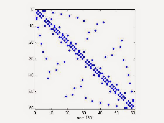
Suppose 'x'  is a sparse matrix, having 60x60 dimensionality. Then  we need to use, the command as "spy(x)" to visualize the sparsity in matlab.
Following matlab's own example of "bucky",
NOTE:  bucky is Connectivity graph of the Buckminster Fuller geodesic dome. Bucky is the 60-by-60 sparse adjacency matrix of the

Commands & Output
>> x=bucky; %generating a 60x60 sparse matrix
>> spy(x) % to visualise the sparsity.

It will pop up a graph plot as,

Bucky Sparsity Visualization

Now playing around with some test more cases of sparsity visualization,
>> spy(speye(10)) %sparsity visualization of 10x10 identity matrix
It will popup the graph plot as,

sparsity visualization of 10x10 identity matrix in matlab

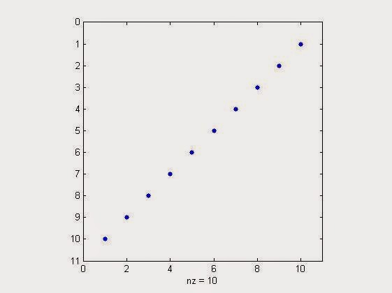
>> spy(flipud(speye(10))) %sparsity visualization of 10x10 identity matrix flipped up side down
It will popup the graph plot as,

%sparsity visualization of 10x10 identity matrix flipped up side down in matlab

Similarly testing it with a colunm vector,
 >> spy(sprand(10,1,0.3)) % generate sparse visualisation plot for a sparse 10x1 column vector with a sparsity of 30%
Result will be,

sparse visualization plot for a sparse 10x1 column vector with a sparsity of 30% in matlab

Many things waiting for you at Digital iVision Labs!

Read More Swapping Rows & Columns of Matrix in MATLAB

Author: Vibhutesh Kumar Singh

An active & prominent author at Digital iVision Labs! Specializing in MATLAB, C++, Arduino, OpenCV, NI Labview, Web Designing & other Electronics stuffs! Just started M.Tech. From IIIT Delhi, looking for excellent PhD Opportunities with prominent researchers. Drop a mail: vibhutesh[at]gmail.com or Follow him at....

Facebook

Twitter

Google+

Linkedin