MATLAB SNR Vs Probability of Symbol Error Curve For M-ary QAM in AWGN channel: Error Probability Curve For M-ary QAM

QAM(Quadrature amplitude modulation) is extensively used in digital data radio & data communications applications. A variety of forms of QAM are available and some of the more common forms include 4QAM, 8QAM, 16 QAM, 32 QAM, 64 QAM & 128 QAM.

The advantage of using QAM is that its higher M-ary type is able to carry more bits of information per symbol, with a very less significant degradation in channel performance. Thus, selecting a higher order format of QAM, the data rate of transmission can be increased.

For the constellation diagram & other advanced information you can get various resources over the internet, you need to just search it with the right keyword.
Now, coming to the MATLAB implementation part.

SNR Vs Probability of Symbol Error Curve For M-ary QAM in AWGN channel: Error Probability Curve For M-ary QAM

%Here we have plotted for the following M-ary schemes, 4,8,16,32,64 & 128-ary QAM.
%different colors have been used to indicate different M-ary plot.
clc
close all
clear all
lc = ['m','r','g','b','k','c'];
%for diffrent color plot for each M-ary
nsample = 1; % number of samples per symbol, default it is 1
M = 4; %starting M-ary number
for i = 1:6
    snr = 0:2:30;
%till 30 dB
    nbits = log2(M); %calculating the number of bits per symbol
    esym = snr + 10*log(nbits) + 10*log(nsample); %energy of symbol
    esyml = db2mag(esym); %converting dB to linear scale
    pe = 4*qfunc(sqrt(3*esyml/(M-1))); %probability of error
    semilogy(snr,pe,lc(nbits-1)) %plotting the error curve
    hold on
    M = M*2;
%doubling the M in M-ary system
end
xlabel('SNR (dB)')
ylabel('Probability of Error')
title('Symbol Error Probability Curve of M-ary QAM')
grid on
legend('M = 4','M = 8','M = 16','M = 32', 'M = 64', 'M = 128')

Result of the above code execution:(Click on the image to Enlarge)
MATLAB SNR Vs Probability of Symbol Error Curve For M-ary QAM in AWGN channel: Error Probability Curve For M-ary QAM
Feel free to comment if you git a better code for it. I will be posting that too as the extension to this article.


0 comments:

Rayleigh distribution PDF & CDF plot in MATLAB using & without using Inbuilt Functions

The Rayleigh distribution, is named after Lord Rayleigh. It is the distribution of the magnitude of a two-dimensional random vector whose coordinates are independent, identically distributed, zero mean normal variables.

The Rayleigh Distribution

Suppose that Z1 and Z2 are normally distributed independent random variables. The magnitude R=Z21+Z22 has the Rayleigh distribution.

The Rayleigh PDF
 It is defined by the following expression: 
The Rayleigh PDF
The Rayleigh CDF
The Rayleigh CDF
Here "σ" may be considered as rms value of the received voltage signal, if seen through a communication engineer point of view.

Rayleigh fading
Rayleigh fading model assume that the magnitude of a signal that has passed through such a communication channel will fade, according to a Rayleigh distribution — the radial component of the sum of two uncorrelated Gaussian random variables.
It is viewed as a justified model for tropospheric and ionospheric signal propagation as well as the effect of heavily cluttered urban environments on wireless communication channel. Rayleigh fading is most applicable when there is no dominant propagation along a line of sight between the 2 communication ends. But if there is, Rician fading will be more applicable.

MATLAB Code for Plotting Rayleigh Distribution PDF & CDF without using the inbuilt function  of Rayleigh PDF & CDF:
%also the mean, variance & median have been calculated in the code
clc;
close all;
clear all;
sig=1;
%RMS value of received voltage signal
r = 0:0.1:10;
%the range of value of 'r'
pdf=(r/sig.^2) .* exp(-r.^2/2*(sig.^2));
% the Rayleigh PDF
figure;
plot(r,pdf,'b')
%Plotting the Rayleigh PDF
title('Rayleigh PDF Plot');
xlabel('r');
ylabel('p(r)');
cdf=1-exp(-r.^2/(2*1));
% the Rayleigh CDF
figure;
plot(r,cdf,'b')
%Plotting the Rayleigh PDF
title('Rayleigh CDF Plot');
xlabel('r');
ylabel('P(r)');
mean=1.2533*sig;
%mean of the Rayleigh distribution
varr=0.4292*(sig^2);
%variance of the Rayleigh distribution
median=1.177*sig;
%median of the Rayleigh PDF

Result of The above Code:
 
Rayleigh distribution CDF MATLAB Plot With σ=1

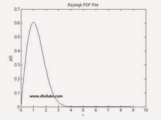
Rayleigh distribution PDF MATLAB Plot With σ=1

The same plot can be obtained by using the MATLAB's inbuilt Rayleigh distribution PDF & CDF function, raylpdf & raylcdf. Just replace the function definition part with the proper formatted raylpdf & raylcdf.
The code after the necessary modification (Now we are using MATLAB inbuilt functions of Rayleigh Distribution PDF & CDF) will look like: [The modification done is denoted by ****]
clc;
close all;
clear all;
sig=1;
%RMS value of received voltage signal
r = 0:0.1:10;
%the range of value of 'r'
pdf=raylpdf(r,sig);
% the Rayleigh PDF ****
figure;
plot(r,pdf,'b')
%Plotting the Rayleigh PDF
title('Rayleigh PDF Plot');
xlabel('r');
ylabel('p(r)');
cdf=raylcdf(r,sig);
% the Rayleigh CDF
figure;
plot(r,cdf,'b')
%Plotting the Rayleigh PDF ****
title('Rayleigh CDF Plot');
xlabel('r');
ylabel('P(r)');
mean=1.2533*sig;
%mean of the Rayleigh distribution
varr=0.4292*(sig^2);
%variance of the Rayleigh distribution
median=1.177*sig;
%median of the Rayleigh PDF

The Result of Above code for plotting the PDF & CDF of Rayleigh Distribution Using MATLAB inbuilt function is:

Rayleigh distribution CDF MATLAB Plot With σ=1

Rayleigh distribution PDF MATLAB Plot With σ=1
Just have a try with different range of 'r' or a different value of sigma.

0 comments:

MATLAB "bertool" : Bit Error Analysis Tool in MATLAB Communication System Toolbox

You might be a communication system designer, or a newbie in communication. While designing or applying any of the modulation scheme with or without modulation for any type of channel you need to have the information of the Bit Error Rate for a particular SNR, so that you can decide on the various parameters of your system (for e.g., transmit power). Or sometime you just want to compare your developed system or scheme with the currently available theoretical references  of the BER values. For that need MATLAB's communication system toolbox has been bundled with a tool, in which you just need to select a few options & there you will get the result you want for the BERs.

So assuming you did already installed MATLAB's Communication System Toolbox, for starting the Bit Error Analysis Tool you just need to type & enter the command in the MATLAB's command window as "bertool".

That will popup a window like this,
The Bit Error Analysis Tool in MATLAB's Communication System Toolbox: BERTOOL
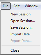
The file menu has some options for the user. 
fILE MENU OF BERTOOL MATLAB
That is, New Session, Open Session, Save Session, Import Data & Export Data. The Export Data, will be enabled when you have already did a simulation, which you can later on import, through, Import Data option.

In the tabs below, the Theoretical Tab, you may be seeing various options, one of them is the Eb/No range setting.
Eb/No Range Set in BERTOOL:  Bit Error Analysis Tool in MATLAB Communication System Toolbox
Eb/No Range Set in BERTOOL:  Bit Error Analysis Tool in MATLAB Communication System Toolbox
If you want it to be in the range -6 to 20 dB you just need to specify it as, -6:20 in the above input box. This will serve as your x-axis while the BER plot has been generated.

Below that, there is also an option to select the channel type, it provides us with three options,
AWGN, Rayleigh, & Rician. After the selection you will get various other options related to these channel that you can tweak in to further control your channel.
Channel Type AWGN in BERTOOL : Bit Error Analysis Tool in MATLAB Communication System Toolbox

Channel Type Rayleigh in BERTOOL : Bit Error Analysis Tool in MATLAB Communication System Toolbox

Channel Type Rician in BERTOOL : Bit Error Analysis Tool in MATLAB Communication System Toolbox

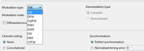
It provides Various options in Modulation Schemes even.
Namely, PSK, DPSK, OQPSK, PAM, QAM, FSK, MSK, & CPFSK.
Modulation Type in BERTOOL:  Bit Error Analysis Tool in MATLAB Communication System Toolbox
Modulation Type in BERTOOL:  Bit Error Analysis Tool in MATLAB Communication System Toolbox
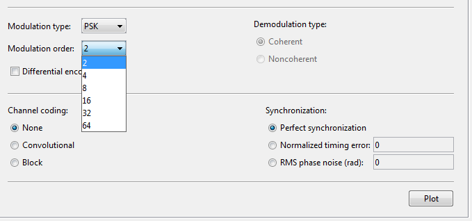
Selection of Modulation Order, in BERTOOL
So, for a M-Ary modulation scene you got various options, i.e., from 2 to 64.
Select & browse through various modulation schemes & you will be seeing various options enabling & disabling with them.
Like while selecting the PSK & OQPSK, you will see an option to enable Differential Encoding to appear & demodulation type option is disabled. And while selecting PAM, QAM,  FSK you will not see any option of Differential Encoding.
Like wise you need to select what your communication system requires.

For Channel Coding part, You need to select Either, None, Convolutional or Block type of Coding.

While selecting the Convolutional coding, you need to specify the trellis polynomial & what decision method you will use while decoding it.

Channel Coding Methods in MATLAB "bertool" : Bit Error Analysis Tool in MATLAB Communication System Toolbox
Another coding type will be the Block Code. Below are the various options available with it.
Block Coding Option in MATLAB "bertool" : Bit Error Analysis Tool in MATLAB Communication System Toolbox

At last to generate a MATLAB BER vs SNR plot just press the button, "Plot".

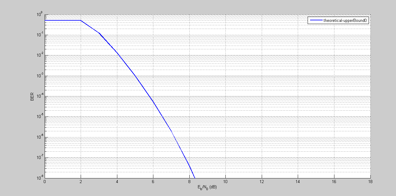
I have selected, to plot from 0 to 18 dB SNR, AWGN Channel. 4-QAM modulation, with convolutional code, hard decision & the Trellis polynomial is represented by, poly2trellis(7, [171 133]). The result is,

BER Plot, MATLAB 4-QAM, AWGN Channel, With Convolutional Coding/Decoding.
So when you run a simulation you get to see something new at the top, which is the data associated with the simulation that you can save, & reload for the next time if you want.
The data after the simulation has completed. MATLAB bertool.
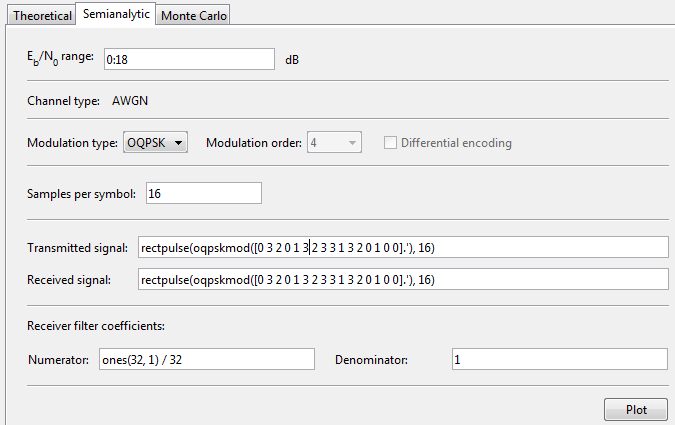
 The semianalytic mode of MATLAB BERtool, has the same functionality, but it gives more flexibility in terms of deciding the bits/symbols to get an analysis of. And additionally the receiver filter coefficient has been added.
The Semianalytic Mode for the BERTOOL MATLAB.
You at last can do, Monte Carlo simulation also in MATLAB's BERTOOL. With various options.
Option of Monte Carlo Simulation in bertool, in MATLAB
So, have a happy day with the BERTOOL of MATLAB. I am sure that this tool will be handy for you, if you need a serious wireless system design.


0 comments:

Eb/No (SNR) Vs BER Curve Plotting for BPSK in AWGN Channel : Error Probability Curve For BPSK

In digital communication, during transmission the bits usually gets altered, i.e., the transmitted '1' is interpreted as '0' & transmitted '0' is interpreted as '1', this constitutes as a bit error. This happens due to various factors, like noise, fading etc. The bit error rate (BER) is the number of bit errors divided by the total number of transmitted bits over a channel. BER although unit-less also expressed in terms of percentage.
E.g., let the transmitted bit sequence:
1 1 1 0 0 0 1 1 1 0
& the received bit sequence:
1 1 0 0 1 0 1 1 0 0 ,
Then the number of bit errors in this case is 3. The BER is 3 incorrect bits divided by 10 transmitted bits, resulting in a BER of 0.3 or 30%.

That was a bit about BER, now something about AWGN channel,
Additive white Gaussian noise (AWGN) is a basic channel model used to study the effect of  random processes that occurs in nature.
  • Its assumed to be 'Additive', so the modelling will be easy.
  • 'White' refers to idea that it has uniform power across the frequency band.
  • 'Gaussian' because it has a normal distribution in the time domain, with average value zero.
The central limit theorem also states that the summation of large number of random processes will tend to have Gaussian or Normal distribution.

MATLAB Implementation:
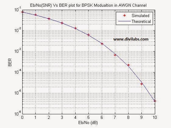
In the given example below, we have generated 100000 bits in order to have enough number of bits to generate a nearly real life curve. Also for each SNR value we have waited for 100 bit errors to occur before proceeding to the other SNR value, as to save the execution time. Later on all the bit errors that occurred are added & the number of bits generated are also added & divided by the former to obtain BER.
In the same curve we have compared the simulation result with the theoretical result as well. 

MATLAB Code for Eb/No (SNR) Vs BER Curve Plotting for BPSK in AWGN Channel:
clc
clear all
close all
bit_count = 100000;
%no. of random bits to be generated for a single shot of BER calculation
SNR = 0: 1: 10; %Range of SNR over which to simulate
for k = 1: 1: length(SNR)
    tote = 0;
%total error bits
    totb = 0;
%total bits
    while tote < 100
%until you get 100 errors
        rbits  = round(rand(1,bit_count));
%generate random bits
        tx = -2*(rbits-0.5);
% BPSK Modulation: Directly to Bipolar NRZ
        N0 = 1/10^(SNR(k)/10);
%noise level
        rx = tx + sqrt(N0/2)*(randn(1,length(tx))+i*randn(1,length(tx)));
        rx2 = rx < 0;
% BPSK demodulator logic at the Receiver
        diff = rbits - rx2;
% Calculate Bit Errors
        tote = tote + sum(abs(diff));
%total errors
        totb = totb + length(rbits); %total bits generated
    end
    BER(k) = tote / totb;
% Calculate Bit Error Rate
end
semilogy(SNR,BER,'*r');
hold on;
xlabel('Eb/No (dB)');
ylabel('BER');
title('Eb/No(SNR) Vs BER plot for BPSK Modualtion in AWGN Channel');
thber = 0.5*erfc(sqrt(10.^(SNR/10)));
% Theoretical BER
semilogy(SNR,thber);
grid on;
legend('Simulated Curve', 'Theoretical Curve');


Result of above Code:
Eb/No (SNR) Vs BER Curve Plotting for BPSK in AWGN Channel

0 comments:

Envelope Detection Using MATLAB for Any time Domain Signal (Thorugh Hilbert Transform)

Envelope Detection Using MATLAB for Any time Domain Signal
The above diagram/plot is of an Amplitude Modulated wave, & we have just found its envelope. This was the result of one of the MATHWORK'S example in simulink to demodulate the AM signal.

Electronically envelope detector is a very simple circuit, consisting of a diode, resistor & capacitor. From ages it has been used to De-modulate the amplitude modulated signals, on the receiver side. The output of the circuit is approximately a voltage-shifted version of the original baseband signal. A simple filter (like a capacitor) can be used to filter out the DC component. In order to get the desired amplitude variation.

That was a little about the circuit implementation of Envelope Detector, but how through a MATLAB code we are going to implement the envelope detection?
Envelope Detection Using MATLAB
The answer lies hidden in the Hilbert Transform. It been a very common and efficient technique for envelope detection. The Hilbert transform is typically implemented as an FIR filter so the original signal must be delayed to match the group delay of the Hilbert transform. This process can be followed by absolute and then peak hold functions.

Another option for detecting the envelope is to use the square root of the energies of the original and the Hilbert transformed signals, as follows :
Envelope = sqrt(Hilbert^2 + signal^2)
In general, this will give similar results to the absolute value technique but can be more run-time efficient.

So, in order to do it, in MATLAB just the simplest way to add this line after the signal of which the envelope has to be calculated.
envelope = abs(hilbert(Signal));
We will show with the help of example,

Demodulating the AM Signal, using Envelope Detection through MATLAB.
clc;
clear all;
close all;

Ac=2; %carrier amplitude
fc=0.5; %carrier frequency
Am=.5; %message signal amplitude
fm=.05; %message signal frequency
Fs=100; %sampling rate/frequency

ka=1; %modulation coefficient

t=[0:0.1:100]; %defining the time range & disseminating it into samples
ct=Ac*cos(2*pi*fc*t); %defining the carrier signal wave
mt=Am*cos(2*pi*fm*t); %defining the message signal
AM=ct.*(1+ka*mt); %Amplitude Modulated wave, according to the standard definition


plot(AM, 'b');
hold on;
envelope = abs(hilbert(AM));
% hilbert transform to calculate the envelope of the signal
plot(envelope, 'r');
hold off


The result is:
Envelope Detection Using MATLAB for Amplitude Modulated Wave (AM Demodulation)
Another similar result we have obtained by applying it to a product of exponential & cosine signal. The code & result as follows:
clc;
clear all;
close all;

Ac=2; %carrier amplitude
fc=0.5; %carrier frequency
Am=3.5; %message signal amplitude
fm=.05; %message signal frequency
Fs=100; %sampling rate/frequency

ka=1; %modulation coefficient

t=[0:0.1:100]; %defining the time range & disseminating it into samples
ct=Ac*cos(2*pi*fc*t); %defining the carrier signal wave
mt=Am*exp(t); %defining the message signal
AM=ct.*mt; %Amplitude Modulated wave, according to the standard definition


plot(AM, 'b');
hold on;
envelope = abs(hilbert(AM)); % hilbert transform to calculate the envelope of the signal
plot(envelope, 'r');
hold off
The result is:
Envelope Detection Using MATLAB for Any time Domain Signal (Thorugh Hilbert Transform)

3 comments:

MATLAB BATMAN Equation Plot

The BATMAN plot has been in news since google has plotted it on its website.

Google BATMAN Plot
Google BATMAN Plot

The plot, itself when taken as a whole, is not a function, as its clear from the above google plot, that it has 2 values of Y-Axis for a single value of X-Axis, & vice versa. Also its clear from the above plot that its a piecewise function, we have plotter the BATMAN head, wings (Upper & Lower part), lover body, etc separately. Thus mathematically it is feasible only when it has to be plotted piece wise.

So, if someone want to plot it, in MATLAB. He has to do like the same thing as done above. And how the MATLAB Batman equations Plot looks like, is given below:
hold on

% Outer wings
f1 = '(x/7)^2 * sqrt(abs(abs(x)-3)/(abs(x)-3)) + (y/3)^2 * sqrt(abs(y + 3/7*sqrt(33))/(y + 3/7*sqrt(33))) - 1';
ezplot(f1,[-8 8 -3*sqrt(33)/7 6-4*sqrt(33)/7]);


% Bottom
f2 = 'abs(x/2)-(3*sqrt(33)-7) * x^2/112 - 3 + sqrt(1-(abs(abs(x)-2)-1)^2) - y';
ezplot(f2,[-4 4]);


% Outer ears
f3 = '9 * sqrt(abs((1-abs(x))*(abs(x)-0.75)) / ((1-abs(x))*(abs(x)-0.75))) - 8*abs(x) - y';
ezplot(f3,[-1    -0.75 -5 5]);
ezplot(f3,[ 0.75  1    -5 5]);


% Inner ears
f4 = '3*abs(x) + 0.75*sqrt(abs((0.75-abs(x))*(abs(x)-.5)) / ((.75-abs(x))*(abs(x)-.5))) - y';
ezplot(f4,[-0.75 0.75 2.25 5]);


% Connect inner ears (flat line)
f5 = '2.25*sqrt(abs(((0.5-x)*(0.5+x))/((0.5-x)*(0.5+x)))) - y';
ezplot(f5,[-0.5 0.5 -5 5]);


% Inner wings
f6 = '6*sqrt(10)/7 + (1.5-0.5*abs(x)) * sqrt(abs(abs(x)-1) / (abs(x)-1)) - 6*sqrt(10)/14 * sqrt(4-(abs(x)-1)^2) - y';
ezplot(f6,[-3 -1 -5 5]);
ezplot(f6,[ 1  3 -5 5]);


% Change line color and width
set(get(gca,'children'),'Color','b','Linew',2)

% Title
title('Batman'); 

 So here is the curious result that you will get after running the above code:
 
MATLAB BATMAN Equation Plot
So just have a try with the code, & if you get something interesting out of it. Just comment back with the code or mail me, I will love to add that also as an extension of this article.


0 comments:

Plotting Reddit dot com Mascot (The Reddit Alien) in MATLAB

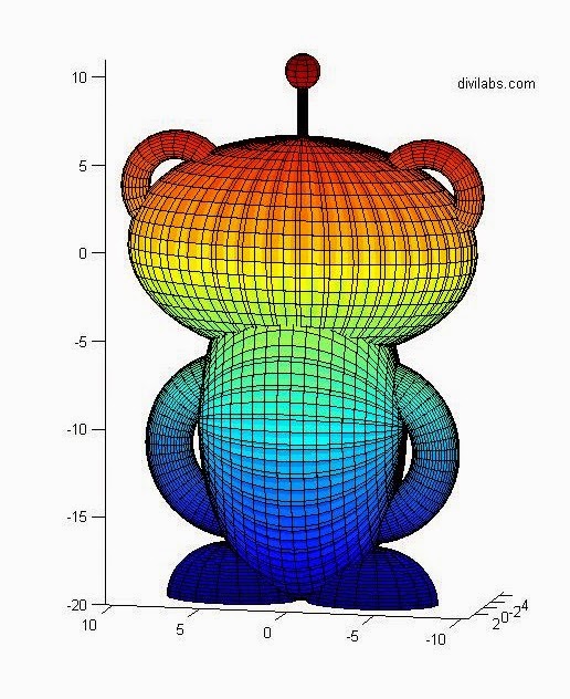
 The idea of plotting Reddit Mascot (The Reddit Alien), had stricken many people before, who were there in reddit & were a member of subreddit, /r/matlab. But it was Nov. 20, 2013 a reddit user, with the profile link http://www.reddit.com/user/Pilotics has posted this image. And this was the MATLAB plot of reddit mascot, the Reddit Alien.
MATLAB Plot of reddit Alien (Reddit MASCOT)
Many have requested him the code of the above plot, but no reply came. But on April 20, 2014, he replied with the code. And the code is:

hold on
view([20 10])

% Head
X=linspace(-2,2*pi,50); Y=linspace(0,2*pi,50);
[Y X]=meshgrid(Y,X);
x=-5.*cos(X).*-2.*sin(Y);
y=-2.*sin(Y).*-2.*sin(X);
z=-sqrt(40).*cos(Y);
surf(x,y,z)


% Antenna
clc % Stalk
R = .25;
Rs = linspace(0, R, 4);
SideH = 5;
Sides = 0:SideH;
Azs = 0:15:360;
[AzMesh1, ZMesh] = meshgrid(Azs, Sides);
XMesh1 = (R * cosd(AzMesh1));
YMesh1 = (R * sind(AzMesh1));
surf(XMesh1, YMesh1, ZMesh+5);
clc % End
R = 1; N = 10;
Ang1 = linspace(0,360 ,N); Ang2 = linspace(-90,90,N);
[Ang1s, Ang2s] = meshgrid(Ang1,Ang2);
X = ([cosd(Ang2s) .* cosd(Ang1s)])*R;
Y = ([cosd(Ang2s) .* sind(Ang1s)])*R;
Z = ([sind(Ang2s)]+10)*R;
surf(X, Y, Z);


% Eyes
clc
for A = -2:4:2
    R = 1.75; N = 25;
    Ang1 = linspace(0,360 ,N); Ang2 = linspace(-90,90,N);
    [Ang1s, Ang2s] = meshgrid(Ang1,Ang2);
    X = ([cosd(Ang2s) .* cosd(Ang1s)]-A)*R;
    Y = ([cosd(Ang2s) .* sind(Ang1s)]-1.75)*R;
    Z = ([sind(Ang2s)]+.75)*R;
    surf(X, Y, Z);
end


% Smile
clc
Space = linspace(-pi,0,50);
[Thetas, Phis] = meshgrid(Space, Space);
Xarr = (cos(Thetas) .* (7 + cos(Phis)))/1.75;
Yarr = (sin(Phis))-3;
Zarr = ((sin(Thetas) .* (1.85 + cos(Phis)))-1);
surf(Xarr, Yarr, Zarr);


% Ears
clc
for A = -9:18:9
    Space = linspace(0,2*pi,25);
    [Thetas, Phis] = meshgrid(Space, Space);
    Xarr = ((cos(Thetas) .* (3 + cos(Phis)))+A)/1.25;
    Yarr = (sin(Phis));
    Zarr = ((sin(Thetas) .* (3 + cos(Phis)))+4)/1.25;
    surf(Xarr, Yarr, Zarr);
end


% Body
clc
X=linspace(-2,2*pi,50); Y=linspace(0,2*pi,50);
[Y X]=meshgrid(Y,X);
z=(-5.*cos(X).*-2.*sin(Y))-10;
y=(-2.*sin(Y).*-2.*sin(X));
x=(-sqrt(35).*cos(Y));
surf(x,y,z)


% Arms
clc
for A = -2.75:5.5:2.75
    Space = linspace(0,2*pi,50);
    [Thetas, Phis] = meshgrid(Space, Space);
    Xarr = ((cos(Thetas) .* (3 + cos(Phis)))+A)/.75;
    Yarr = (sin(Phis));
    Zarr = ((sin(Thetas) .* (3 + cos(Phis)))-8.5)/.75;
    surf(Xarr, Yarr, Zarr);
end


% Feet
clc
for A = -4:8:4
    X=linspace(-2,2*pi,25); Y=linspace(pi,pi/2,25);
    [Y X]=meshgrid(Y,X);
    x=(-5/2.*cos(X).*-3/2.*sin(Y))-A;
    y=(-3/2.*sin(Y).*-3/2.*sin(X));
    z=(-sqrt(10).*cos(Y))-20;
    surf(x,y,z)
end


text(-8, -4, 9, 'divilabs.com');

axis equal
hold off   


The code looks, very complicated, as it deals with the geometry & the plane orientation. But its working fine. So here is the result of our simulation of the above MATLAB code to plot the reddit alien.
Plotting Reddit dot com Mascot (The Reddit Alien) in MATLAB
Plotting Reddit dot com Mascot (The Reddit Alien) in MATLAB Front View
Plotting Reddit dot com Mascot (The Reddit Alien) in MATLAB
Plotting Reddit dot com Mascot (The Reddit Alien) in MATLAB Back View
So just copy the code above, & let your imagination work to get various changes to it.

Special thanks & congrats to the user @Politics for this brilliant piece of work.


0 comments:

Building a Simple GUI Interface in MATLAB (guide)

Yes, building a simple GUI interface through MATLAB is possible. Just like in Visual Basic or Visual C++, you have a drag & drop feature of buttons, text boxes etc, & then you just need to program them in order to define their functionality. If you want to export it as a standalone executable file, you can even do that. But just like the other languages the application build with MATLAB will require its runtime, to be pre-installed.

So, the GUI interface builder for the MATLAB is known by the name "GUIDE". The fullform of GUIDE is "Graphical user interface design environment".

As the MATLAB official help document states about it:
guide is both a directory and a function.
    Calling guide by itself will open the guide Quick Start Dialog where you can choose to open a previously created GUI or create a new one from templates.
guide(filename) opens the FIG-file for editing where you can build up the GUI & related function.

* Just type in the command window with the command & you will see a pop-up appearing like this.
Guide Quick Start Box in MATLAB
* Select the "Blank GUI" option, which is also being selected by default.
* Then press OK & you will see a GUI workspace being opened up in front of you.

GUI building workspace in MATLAB: guide


      * In left hand side there are many types of button interfaces are there. As according to your requirement pick any button and drop in grid area.

NOTE: There are two interfaces in GUI. One is figure and other one is MATLAB code.


Lets take an example, We just want to build a simple GUI that prints your name by a click of button which is present in the GUI.

STEP 1: Take two push buttons & drag them up in the grid box as shown in the above figure.
STEP 2: Tale one static text box & drag it, over the grid box.
STEP 3: Left click on any button (that you have just got in the grids) and go to property inspector. By the help of this you can change various properties of it like name, color, font size etc.
STEP 4: Clear the section of "static text" box by clearing string in property inspector.
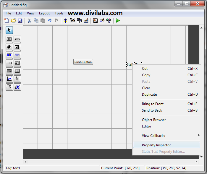


Changing the properties of various objects in MATLAB GUI through Property Inspector
STEP 5: Optional (You can change the size of the button, by dragging the corner points of the button bounding box)
STEP 6: Drag another button (Optional, depends upon your requirement)
Now the resultant GUI will Look like this:
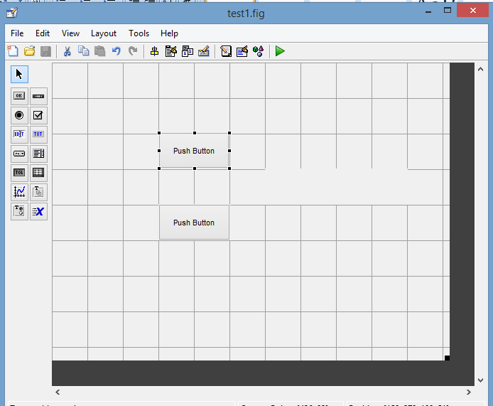
GUI Development in MATLAB
STEP 7: Now the crucial step, go to the "editor" (Right Click on the grid boxes & Select editor) to change in the call back function of the button, which will tell them what to do. It will ask you to save the file with the extension ".fig". Save it & then it will automatically opens the MATLAB editor window, there you have to make changes in the code in order to get the things work.

GUIDE editor option
GUIDE editor option
Here is, what we did in our case (The changes done & added are in BOLD):


function varargout = test1(varargin)
% TEST1 MATLAB code for test1.fig
%      TEST1, by itself, creates a new TEST1 or raises the existing
%      singleton*.
%
%      H = TEST1 returns the handle to a new TEST1 or the handle to
%      the existing singleton*.
%
%      TEST1('CALLBACK',hObject,eventData,handles,...) calls the local
%      function named CALLBACK in TEST1.M with the given input arguments.
%
%      TEST1('Property','Value',...) creates a new TEST1 or raises the
%      existing singleton*.  Starting from the left, property value pairs are
%      applied to the GUI before test1_OpeningFcn gets called.  An
%      unrecognized property name or invalid value makes property application
%      stop.  All inputs are passed to test1_OpeningFcn via varargin.
%
%      *See GUI Options on GUIDE's Tools menu.  Choose "GUI allows only one
%      instance to run (singleton)".
%
% See also: GUIDE, GUIDATA, GUIHANDLES

% Edit the above text to modify the response to help test1

% Last Modified by GUIDE v2.5 05-Apr-2015 01:53:56

% Begin initialization code - DO NOT EDIT
gui_Singleton = 1;
gui_State = struct('gui_Name',       mfilename, ...
                   'gui_Singleton',  gui_Singleton, ...
                   'gui_OpeningFcn', @test1_OpeningFcn, ...
                   'gui_OutputFcn',  @test1_OutputFcn, ...
                   'gui_LayoutFcn',  [] , ...
                   'gui_Callback',   []);
if nargin && ischar(varargin{1})
    gui_State.gui_Callback = str2func(varargin{1});
end

if nargout
    [varargout{1:nargout}] = gui_mainfcn(gui_State, varargin{:});
else
    gui_mainfcn(gui_State, varargin{:});
end
% End initialization code - DO NOT EDIT


% --- Executes just before test1 is made visible.
function test1_OpeningFcn(hObject, eventdata, handles, varargin)
% This function has no output args, see OutputFcn.
% hObject    handle to figure
% eventdata  reserved - to be defined in a future version of MATLAB
% handles    structure with handles and user data (see GUIDATA)
% varargin   command line arguments to test1 (see VARARGIN)

% Choose default command line output for test1
handles.output = hObject;

% Update handles structure
guidata(hObject, handles);

% UIWAIT makes test1 wait for user response (see UIRESUME)
% uiwait(handles.figure1);


% --- Outputs from this function are returned to the command line.
function varargout = test1_OutputFcn(hObject, eventdata, handles)
% varargout  cell array for returning output args (see VARARGOUT);
% hObject    handle to figure
% eventdata  reserved - to be defined in a future version of MATLAB
% handles    structure with handles and user data (see GUIDATA)

% Get default command line output from handles structure
varargout{1} = handles.output;


% --- Executes on button press in pushbutton1.
function pushbutton1_Callback(hObject, eventdata, handles)
% hObject    handle to pushbutton1 (see GCBO)
% eventdata  reserved - to be defined in a future version of MATLAB
% handles    structure with handles and user data (see GUIDATA)
set(handles.text1,'string','vijay sharma');

% --- Executes on button press in pushbutton2.
function pushbutton2_Callback(hObject, eventdata, handles)
% hObject    handle to pushbutton2 (see GCBO)
% eventdata  reserved - to be defined in a future version of MATLAB
% handles    structure with handles and user data (see GUIDATA)
set(handles.text1,'string','vibhutesh');
 

Step 8: Now Run it, you can see a play button in the MATLAB's GUI building Interface, just click once & it will execute your GUI.
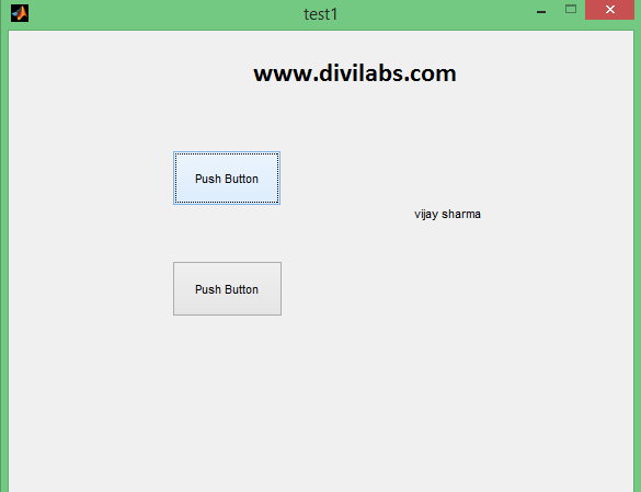
GUI Designed in MATLAB with 2 Buttons & a Static Text Box to Display the Output


Press push button. And see the output!

NOTE: In MATLAB GUI all variables to be displayed should be in string Data Type. So if you taking and number so change it into string.

0 comments: