Calculating & visualizing the Perceived Brightness of a Color Image (RGB) in MATLAB

Calculating the Perceived Brightness of a Color Image (RGB) in MATLAB  or in simple words,
calculating the brightness of an RGB color image.

Before implementing it in matlab, we must know the conversion formula,

RGB -> Luma conversion formula. (more weight-age to green since our eyes are more sensitive to green color.)

Photometric/digital ITU-R: 
(Here 0.2126+0.7152+0.0722=1) 
(Source: en.wikipedia.org/wiki/Relative_luminance)
 Y1 = 0.2126*R + 0.7152*G + 0.0722*B
 
Digital CCIR601 (gives more weight to the R and B components):
(Here 0.299+0.587+0.114=1)
(Source: www.w3.org/TR/AERT)
Y2 = 0.299*R + 0.587*G + 0.114*B
 
If ready to trade accuracy with performance, there are two approximation formulas above two:
(Source : Franci Penov answer )
Y1a = 0.33*R + 0.5*G + 0.16*B 
or Y1a = (R+R+B+G+G+G)/6

Y2a = 0.375*R + 0.5*G + 0.125*B  
or Y2a = (R+R+R+B+G+G+G+G)/8
 

Our Test Image is an RGB image: 225x609 in size
Our Test Image is an RGB image:
Our Test Image is an RGB image 225x609 in size

Suppose we have read the above image through imread( ) function & stored it in a variable named 'x' .
>> x=imread('image.jpg'); %assuming that this image lies in working directory & named "image"

now size(x) will give result as,
ans =   225   609     3 

NOTE: The third element displaying a value of '3' denotes the presence of 3 planes of 225x609 matrix. 1st of which the red (R) plane (designated by value 1 in the 3rd index of x), 2nd is the green(G) plane (designated by value 2 in the 3rd index of x) & 3rd is the blue (B) plane (designated by value 3 in the 3rd index of x) .

In order to access three color planes separately, type your formula like this x(:,:,1) or x(:,:,2) or x(:,:,3). See more about this at: Using MATLAB, Extracting individual Red, Blue & Green (RGB) planes, From a RGB Image, With Code

Now how to apply above three formulas?

Applying Y1 = 0.2126*R + 0.7152*G + 0.0722*B in MATLAB our command will look like,

>> Y1=0.2126*x(:,:,1)+0.7152*x(:,:,2)+0.7152*x(:,:,3);
%to access a particular pixel luma/brightness value calculated by above formula use the command as,

>>Y1(200,200)
ans =  116 

%thus perceived brightness at (200,200)pixel location is 166 in a scale of 255.

% Now since its also stored as an image we can visualize the Brightness values of the image as,

>>imshow(Y1)

The above 2 lines of code will result in another image having a single luma plane, which look like this.
Perceived Brightness of a Color Image (RGB) in MATLAB  by Formula 1
Perceived Brightness of a Color Image (RGB) in MATLAB  by Formula 1

Applying Y2 = 0.299*R + 0.587*G + 0.114*B in MATLAB our command will look like,

>> Y2=0.299*x(:,:,1)+0.587*x(:,:,2)+0.114*x(:,:,3);
>>imshow(Y2) % to see visualize the brightness
 
Perceived Brightness of a Color Image (RGB) in MATLAB  by Formula 2
Perceived Brightness of a Color Image (RGB) in MATLAB  by Formula 2

The above image came to be more darker than Y1 case, due to the fact more weight-age is distributed among R & B value than G.


0 comments:

How to Visualize Sparsity of a Matrix or a Vector in MATLAB?

So, what is sparse signal/matrix/vector? Their generation & use in Matlab refer the link of our previous article, Creating & Using Sparse Matrix & Vectors in MATLAB - Concepts & Examples.

Now its time to visualize the sparsity of generated or received signal/vector/matrix. But why there is a need of visualization?
The actual need arises when we want to see where the energy is concentrated  in the received or generated vector/matrix. If the matrix/vector is sparse then there are very few percentage of non-zero elements, thus energy will be more concentrated to those elements.

The command we will use for this purpose is spy( ). Remember this command has got its place at Digital iVision Labs, earlier also in the article : Unusual Commands of MATLAB. It will give output as, when used without any parameters or function.
Spy Command without any parameter
Now coming towards the topic of visualizing sparsity.
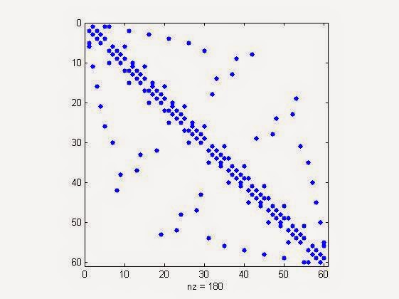
Suppose 'x'  is a sparse matrix, having 60x60 dimensionality. Then  we need to use, the command as "spy(x)" to visualize the sparsity in matlab.
Following matlab's own example of "bucky",
NOTE:  bucky is Connectivity graph of the Buckminster Fuller geodesic dome. Bucky is the 60-by-60 sparse adjacency matrix of the

Commands & Output
>> x=bucky; %generating a 60x60 sparse matrix
>> spy(x) % to visualise the sparsity.

It will pop up a graph plot as,
Bucky Sparsity Visualization
Now playing around with some test more cases of sparsity visualization,
>> spy(speye(10)) %sparsity visualization of 10x10 identity matrix
It will popup the graph plot as,
sparsity visualization of 10x10 identity matrix in matlab
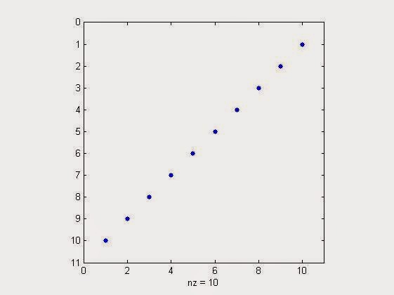
>> spy(flipud(speye(10))) %sparsity visualization of 10x10 identity matrix flipped up side down
It will popup the graph plot as,

%sparsity visualization of 10x10 identity matrix flipped up side down in matlab

Similarly testing it with a colunm vector,
 >> spy(sprand(10,1,0.3)) % generate sparse visualisation plot for a sparse 10x1 column vector with a sparsity of 30%
Result will be,
sparse visualisation plot for a sparse 10x1 column vector with a sparsity of 30% in matlab
sparse visualization plot for a sparse 10x1 column vector with a sparsity of 30% in matlab
Many things waiting for you at Digital iVision Labs!

Read More Swapping Rows & Columns of Matrix in MATLAB


0 comments: